Pre-processing large datasets with Excel, HeidiSQL and MariaDB.
The first dataset I opened was from September 2010. When I said ‘opened’, I meant I tried to open it with Notepad. ‘Opening a text file with little over 4GB data is not possible with Notepad’ was the first lesson I learned working with a large datafile. You understand how much of a novice I was? Of course I had to find another program. Luckily I had the Oxygen XML editor on my computer which at least allowed me to open the file, but it was not suitable for working with, let alone pre-processing the data. I turned once again to my programming colleagues for aid. What would be useable? After contemplating several options one of my colleagues suggested I’d use MariaDB, a relational database made by the original developers of MySQL (and open source). Its Windows version came with the HeidiSQL interface which proved very useful for a novice like I was. A bonus for me was that SQL was a language I was already familiar with because of the WCT database. I was just getting skilled in querying that database when I started this project. So installing and making my own database in a SQL environment nicely complemented my existing skills.
After installation I had a database, an interface and some programming knowledge with which I could use both.
Pipeline with room for errors
Because this was my first major researching project for the web archive, I formulated a workflow that had room for errors. If I messed up one particular step, I wanted to be able to return to the previous steps. And in case of total disaster, I had the possibility to start again from scratch. To this end I created a pipeline that loaded a dataset, generated statistics and then pre-processed the data while keeping the previous steps and original data. The original raw datafile was never edited so I could keep on using it.
Let us start at the beginning: creating the database tables. Creating tables in HeidiSQL is simple and does not require writing code. The HeidiSQL interface allows you to create a table and add columns through its interface. It will write the code belonging with it for you. You can then set the datatype and length for each column. As you can see below I ended up with a varchar column for my URL-columns with 2000 characters. Some URLs turned out to be very long. I suppose that after pruning them this amount could be reduced. This applies to other columns as well. The Type_URL, TR_nr and TI_nr columns for example could easily work with shorter lengths. Type_URL had either ‘anchor’ or ‘embed’ in it, so a length of seven characters would suffice. But this is all hindsight of someone who now has more experience!
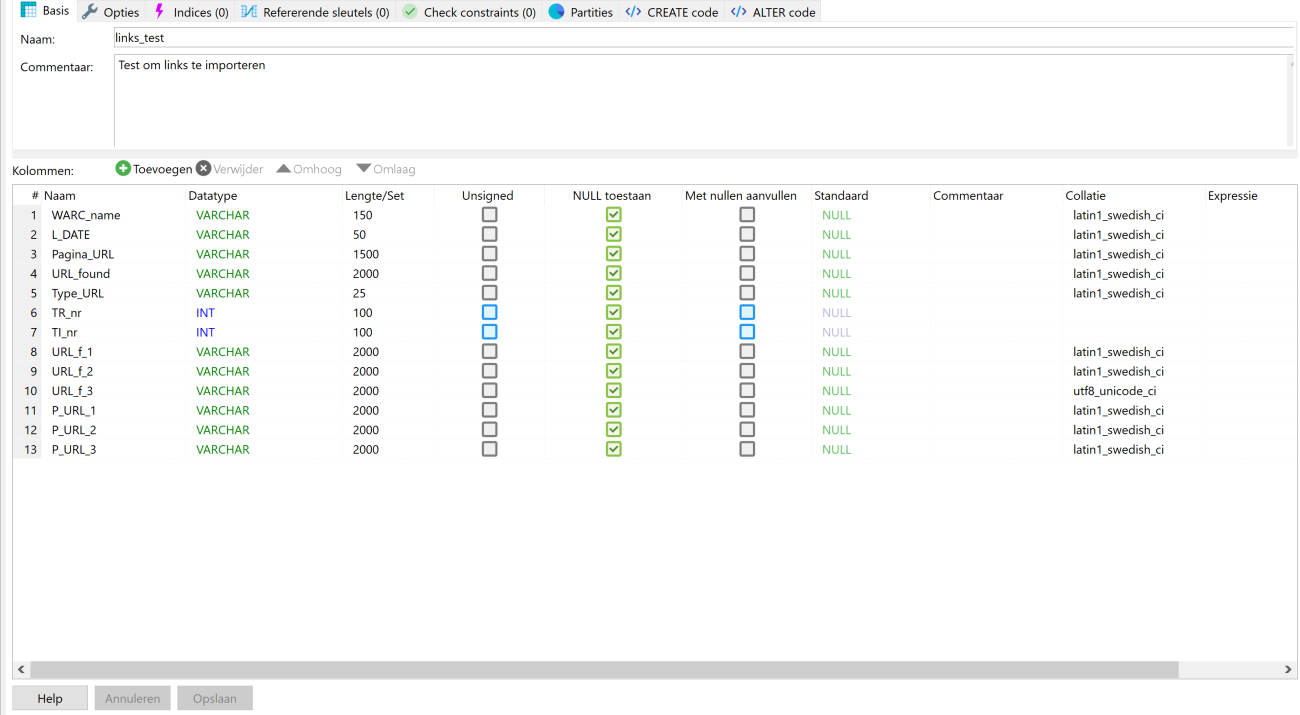
Figure 1. HeidiSQL table settings.
After creating the table I started writing SQL queries. The code I made is separated into four main parts:
- Importing the raw datafile and WCT data
- Checking the metadata and statistics (making checksums)
- Pruning domains
- Exporting data for Gephi
I also made some search-, select- and delete queries to find specific parts within the larger dataset.
Importing issues

Code 1. Importing the dataset.
The first time I imported a dataset, the columns were still separated with spaces. This was not workable because a lot of URLs contained spaces. The URLs were consequently being put into several columns instead of just the one. After replacing the separating sign to tab, ‘load data local’ worked perfectly. However, I needed to increase the URL-columns to 2000 characters (I started out much lower) because the URLs turned out to be very long.
I also retrieved some data from the WCT in a .csv form which I added into two different tables: one for the target record metadata (named wct_tr) and one for the target instance metadata (wct_ti). Both tables were again created through the HeidiSQL interface. HeidiSQL also has an import function for csv’s, so adding this data into the table went very smooth without the need for me to write additional code. I only needed to make sure that it skipped the first row (containing the column-names) and that the csv-columns aligned with the SQL-columns. All tables contained the unique target record or target instance ID’s so joining them through a JOIN query to the links_test table was possible.
I now had three tables filled with all kinds of data ready for the next step.
Checking metadata and making checksums
Before I started processing the data, I checked if I’d gotten the data I was looking for. As mentioned in the previous post, I always checked L_DATE (the warc_date) because I thought this was the time a harvest had started instead of the date that a specific resource was harvested. HeidiSQL lets you sort columns in its interface. So during the first version of my research I sorted the L_DATE column and removed records with an October date through the HeidiSQL interface. Later I rectified this and left the records in the datasets. In future research I would do it differently: I would connect the wct_ti table with the links_test table and check this way if the ti_start_time was accurate. The same approach is possible when one would wish to analyse a specific collection. You could connect the wct_tr table with the links_test table and check if all results have the collection label you were looking for.
After checking if I had gotten the data I was looking for, I made sure to get some relevant statistical numbers with some simple counting queries. I for example counted how many URLs found were an anchor and how many an embedded link. Of course I also checked how many URLs had been found in total (per dataset). But most interesting were the statistic about how many harvests (target instances) had provided results and if there were target records that had run twice in September.
Counting total number of URLs in the dataset:

Code 2. Total URLs found.
This is the most important checksum number needed for step three; the pruning of the domains. Every time I cropped a part of the URL I made sure it was done this amount of times. This method worked for me because I filled out a new column for each pre-processing step. Verifying this checksum number made sure the step was at least done for each row and each column had been fully filled. Because of this checksum I, for example, quickly found out my cutting-away-the-page code did not worked on rows that did not contain the a ‘/’ sign.
| Year | Rows / URLs found |
|---|---|
| 2010 | 14.738.323 |
| 2013 | 8.768.023* |
| 2016 | 18.743.292 |
| 2019 | 40.185.083 |
* I never did figure out why 2013 had so little ‘rows found’.
Results found from…
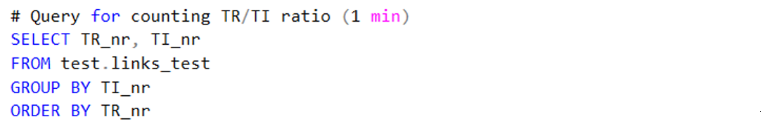
Code 3. Piece of code used to identify which target records had multiple target instances. If a target record appeared in multiple rows in the result, it harvested multiple times in September.
Because our archive is a selective archive I can also check if websites are appearing multiple times in the dataset through counting the ID’s. I can check this by comparing the number of target records present with the number of target instances present. If a website only harvested one time in September, it should only have one target instance number per target record number. As you can see below though this is not the case. Some target records therefor harvested multiple times in the month September. This means that without any deduplication this website will be present multiple times in the dataset, probably causing it to be over-represented in the final visualisation. I have not deduplicated this dataset at present, but should have done so. If I had deduplicated the dataset the number of target records and target instances present in the dataset should have been the same (one record should only have one instance).
| Number of... | 2010 | 2013 | 2016 | 2019 |
|---|---|---|---|---|
|
Target records present in dataset |
600 | 768 | 905 | 1.313 |
|
Target instances present in dataset |
602 | 802 | 944 | 1.352 |
| Harvests present in the dataset | TI per TR 2010 | TI per TR 2013 | TI per TR 2016 | TI per TR 2019 |
|---|---|---|---|---|
| 1 | 598 | 762 | 896 | 1277 |
| 2 | 2 | 5 | 6 | 33 |
| 3 | 0 | 0 | 1 | 3 |
| 4 | 0 | 0 | 1 | 0 |
| 29 | 0 | 0 | 1 | 0 |
| 30 | 0 | 1 | 0 | 0 |
Cropping hyperlinks to domains
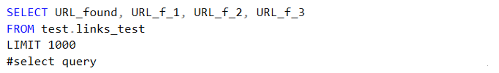
Code 4. Select query for pruning columns
Once I had the database complete and some statistics ready, work could start on pre-processing the hyperlinks. For both URL found and the page-URL the process was the same. The URLs needed to be cropped back to whole domains. So:
https:// www. kb.nl/en/organisation/research-expertise/long-term-usability-of-digital-resources/web-archiving
would need to be brought back to
kb.nl
This needed to be done while maintaining what happened during each step. If in later steps it turned out something went wrong, I would be able to pinpoint where it went wrong (and if it was a processing error or an irregularity in the data). So I chose to place the data in a new column with each cropping step instead of making just one query that did all in one go.
- First I would remove all http:// and https:// strings by cutting away everything left of the double forward slash (‘//’).
- Secondly I removed the pages by cutting everything right of a single forward slash (‘/’). As mentioned above I wrote two parts for cutting away the page: one where the column contained an ‘/’ it would cut away the page and one where the column did not contain an ‘/’ it would just copy the content.
- And finally I removed the ‘www.’ string.
This provided me with an acceptable result. It was not perfect but it worked well enough to continue the project.
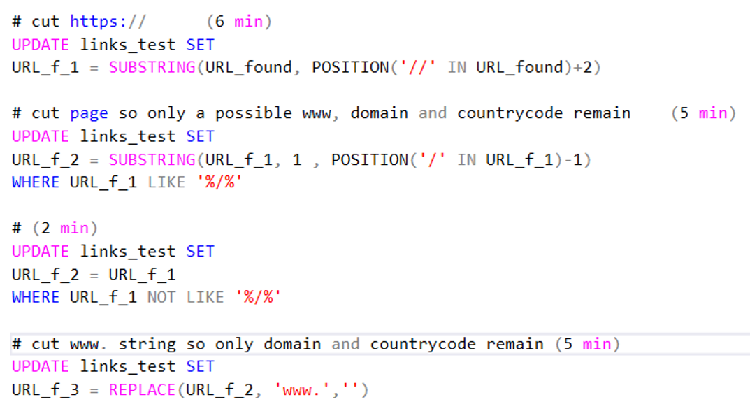
Code 5. Pruning code. Time indication (5 min for example) belongs with 2013 dataset. Bigger sets took a while longer.
There were several types of URLs that did not cropped well with this method. One was the ‘javascript’ anchor, found in every dataset. For example:
- Javascript://Print this Event
- javascript://
This URL was found, but cropped incorrectly because of the first cropping step. Because of cutting the strings on the double forward slash ‘javascript’ was cut away, leaving the cell empty or with just ‘Print this Event’. This goes for similar built URLs as well. All URLs built differently than ‘https://’ or ‘http://’ strings were probably processed incorrectly. Other examples I encountered were ‘file:///C’, (or E or D) anchor and embed hyperlinks and ‘whatsapp://send’ anchors.
The ‘www.’ cutting point could also do with an improvement should I preform a similar research in the future. At present it is case sensitive: so it does not remove for example ‘Www.’. Then we also have the www2., www3., etc. which are processed incorrectly. These URLs are hostnames or subdomains used to identify closely related websites and are typically used for server load balancing. In the 2019 edges dataset there are roughly 1.600 edges were the ‘www.’ is not pre-processed correctly. On a total of roughly 330.000 edges, this is not perfect, but workable for a proof-of-concept project.
Exporting data
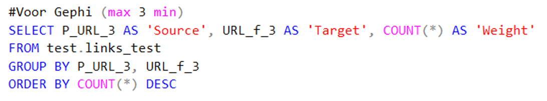
Code 6. Code used to make the dataset with all results for Gephi.
After the domains had been pruned, the edges datasets could be made. For the purpose of this research I generated three datasets: one representing all results grouped together, one with only the embedded hyperlinks and one with only the anchor results. All datasets had three columns that could be directly imported in Gephi (I gave them recognisable titles the program understood) if desired. Source (pre-processed URL on which a link was found), Target (pre-processed links that were found) and Weight (how many times a source had found a target). This gave the following data (example): kb.nl, dbnl, 7. Or in words: kb.nl points seven times to dbnl.nl in this dataset. Please note that the export format was a .csv file!
| 2010 | 2013 | 2016 | 2019 | |
|---|---|---|---|---|
| Edges All | 84.058 | 120.121 | 162.070 | 331.696 |
| Edges Anchor | 82.674 | 117.524 | 158.307 | 323.122 |
| Edges Embed | 2.302 | 4.062 | 5.579 | 12.638 |
Close reading data from a distance
Before I ingested the data in Gephi I had to take one final step. I close read my data in Excel. Why? Do you ask. Well, I like to know exactly what is in my dataset: what worked, what did not work, why it did not work. This is how I found out about the Javascript and Whatsapp for example. I created a nice cycle between identifying anomalies in my Excel sheet (why is this cell containing only a strange string), in relation to the HeidiSQL pre-processing columns (in which pre-processing step did this anomaly occur?).
Code 7a. Search query to find a string.
These little search queries also allowed me to make smaller datasets which I could then export and visualize.
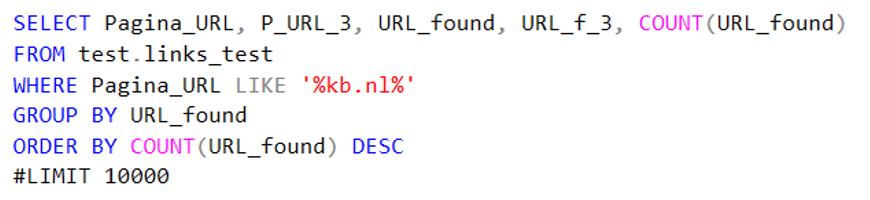
Code 7b. Column specific search query to find a domain.
After exploring the datasets I decided to delete the following edges in all datasets (when found):
- Edges with the target field being empty (this meant that rows containing a space remained).
These edges were not suitable for Gephi as information was missing.
- Edges pointing to themselves
These edges were not relevant for the research I was doing (researching outward pointing links in the web collection).
- Edges only containing http of www
Pointless for this research as it was not a full domain.
- Edges containing the string ‘subject=’
Only occurred in 2016 for one domain. These were all mailto links. By removing them I lessened the import load for Gephi.
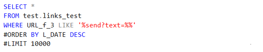
- Edges containing the string ‘send?text=’
These were all Whatsapp edges that had been wrongly pre-processed. By removing them I again lessened the import load for Gephi especially in 2019.
I also found out a lot of target-domains having an ‘ on the end of their string. I adjusted this as well (kb.nl’ became kb.nl). After this intervention the datasets were ready to be visualized in Gephi!
| 2010 | 2013 | 2016 | 2019 | |
|---|---|---|---|---|
| Edges HeidiSQL | 84.058 | 120.121 | 162.070 | 331.696 |
| Edges after removal edges | 83.725 | 119.589 | 153.317 | 291.304 |
| Edges were ' was removed | 770 | 745 | 2.671 | 10.303 |
Knowing your data
I think of all my work, this part is the most important. It is probably the same with almost every research. You spend weeks pre-processing your data and then only a couple of days visualizing them. Your visualizations are only as good as your data, so I think it is important to understand how your data is constructed even if you do not necessarily make them (as I have done).
My next blogposts will be about working with Gephi and the consequences of my pre-processing steps. First I will end the workflow part of these posts and go into detail how I worked with Gephi as a tool. The following blogpost is the start of the lessons learned and result part. I start this off by delving into the analysis of the Gephi visualizations and finding out what happened to Hyves (a now offline Dutch Social Media website).
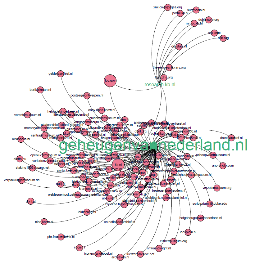
Figure 2. Little teaser of upcoming link visualizations.

Related
Previous: Let's get some data - Link analysis part 1
Next: Working with Gephi - Link analysis part 3
Glossary
Anchor link – for our research these are hyperlinks with a href tag (<a>, <link>, <area>)
Embedded link – for our research these are hyperlinks without href tag (<img>, <script>, <embed>, <source>, <frame>, <iframe> and <track>)
HeidiSQL - lets you see and edit data and structures from computers running one of the database systems MariaDB, MySQL, Microsoft SQL, PostgreSQL and SQLite. For our research we use MariaDB.
Gephi - a visualization and exploration tool for all kinds of graphs and networks. Gephi is open-source and free.
MariaDB - a relational database made by the original developers of MySQL, open source.
Target Record (or Target) – Contains overarching settings such as schedule frequency (when and how often a website is harvested) and basic metadata like a subjectcode or a collection label.
Target Instance - is created each time a Target Record instructs Heritrix to harvest a website. Contains information about the result of the harvest and the log files.
WARC – file type in which archived websites are stored. The KB archive consists of WARC and its predecessor ARC files. This project was done for both types of files.
WCT – Web Curator Tool is a tool for managing selective web harvesting for non-technical users.
Web collection – For the KB: they have a selective web archiving policy were they harvest a limited number of sites. You can find an overview of all archived websites at the KB on their FAQ page [Dutch].